A system to generate realistic and difficulty-graded hiking trail networks on top of terrain surfaces.
My Master’s thesis, titled Analysis and generation of hiking trail networks from terrain metrics, was part of the larger SENDA project from the Research Center for Visualization, Virtual Reality and Graphics Interaction (ViRVIG). Development started during a university course in UPC in early 2023, then intensified when I started working part-time in ViRVIG in February 2024.
Overview
SENDA (Simulation and visualization of Erosion and Nature Degradation due to Anthropogenic activities) is an ambitious project that aims to model the impact of human outdoor activities in nature. It is divided into several phases and subprojects, that can be developed more or less independently.
My task was to develop a system that, given a terrain surface, would generate a set of interconnected hiking trails resembling those seen in real life. This would then be used to guide the simulation of agents, and measure their impact on the natural environment.
This also required an in-depth study of terrain metrics and their effect on the trajectory of real mountain trails. The most relevant terrain metrics (terrain slope, path slope, surface roughness and the topographic position index) are used to condition the path generation.
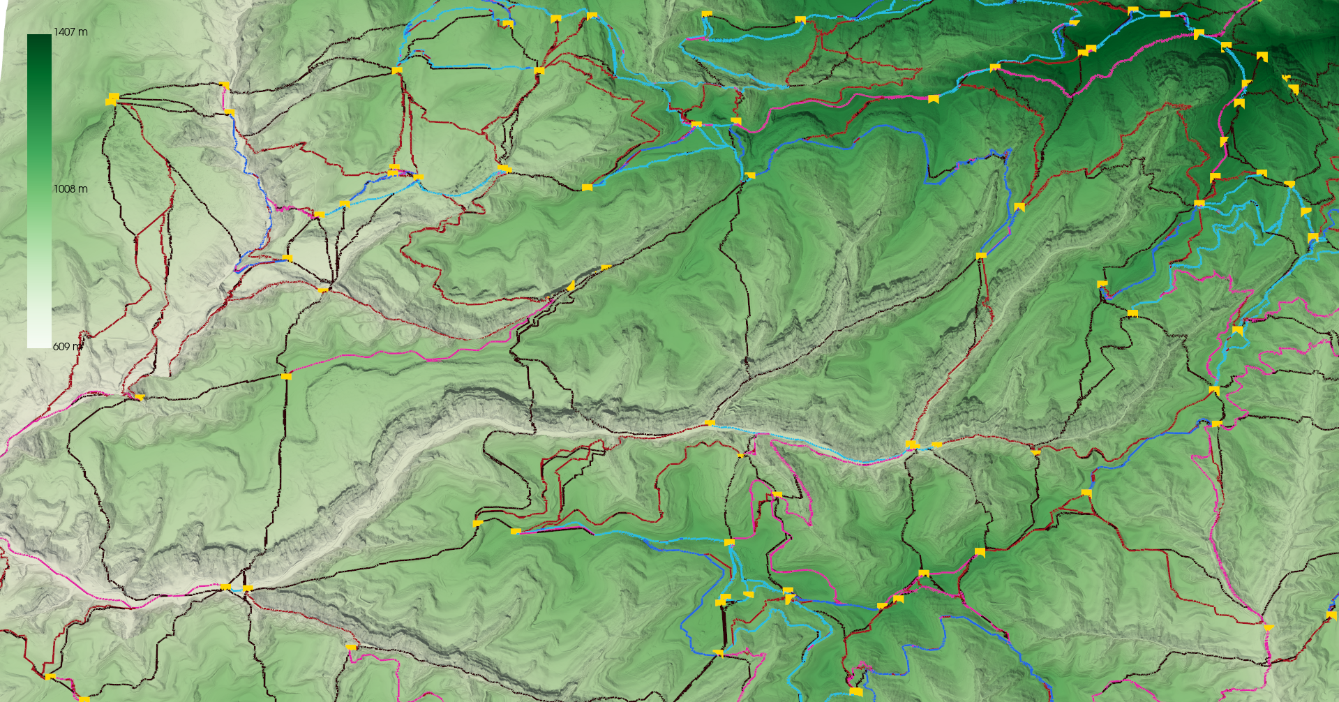
The final result is a set of hiking trails, with possible intersections and mergings, that connect a collection of relevant Points of Interest (PoIs) of the terrain, such as viewpoints, camping sites, parkings, etc. Each trail is labeled according to their difficulty; labels follow the SAC scale.
Data sources
We used OpenStreetMap to download public data regarding existing mountain trails (and their difficulty level, if available) and PoIs for a given region. The final system also allows the use of synthetic data, but we use trails from the real world to train the generator.
Our study focused on the country of Switzerland. This is because of their high-quality mapping and labeling in OpenStreetMap, but also because they offer public and high-resolution Digital Elevation Models in the swissALTI3D dataset. Again, the system can work with other terrains (3D elevation data is available worldwide, with more or less resolution depending on the region), but good quality and uniform data facilitates the study.
My contribution
The work developed in this project can be split into three phases, each an interesting project of their own, with different methodologies and results, but depending on the results from the ones before.
1. Difficulty classification
Determining the difficulty of a trail from the terrain.
The goal of this phase was to analyze which terrain metrics are more relevant when it comes to determining the path that a mountain trail follows, as well as the difficulty.
Generating the dataset
The biggest workload in this phase was the generation of the dataset. This involved bulk downloading and aggregating data from multiple sources (mainly OpenStreetMap and swisstopo, amounting to >50 GBs of terrain data), and coming up with optimized techniques for efficiently computing the terrain metrics for each trail.
The process still took around 2 days to compute in a powerful PC.
Classification
The result of the previous task is a uniform dataset with a collection of paths (~50k), each labeled with a SAC scale number and a value for each of the analyzed terrain metrics (38 in total).
We tested different options for classifiers. In the end we setteled to use a large set of random forest classifiers to compensate for class imbalance.
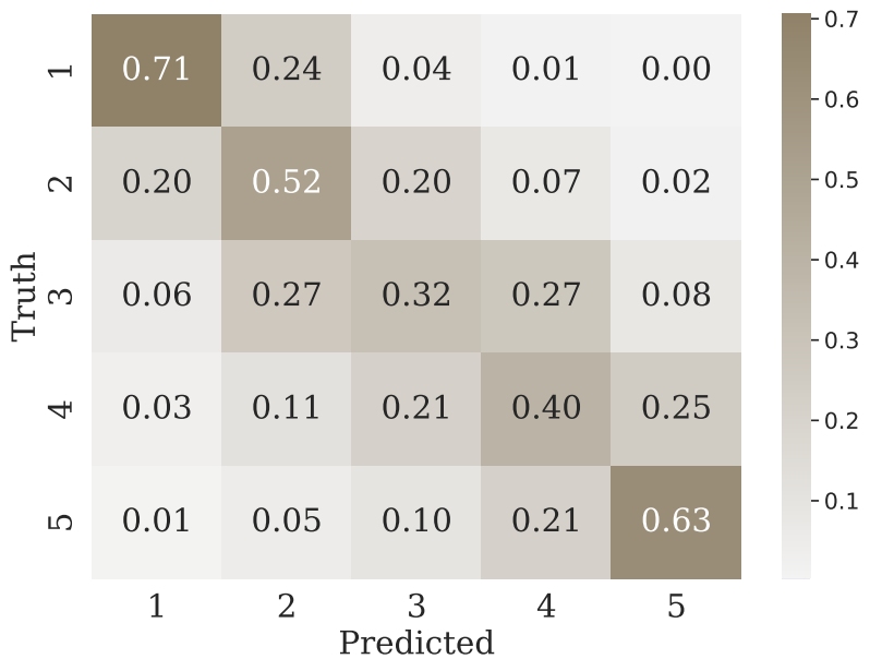
If we tolerate off-by-1 errors (a common practice, since the original labels are very subjective to begin with) we are able to obtain ~89% accuracy. With some setups tailored specifically to this dataset we obtained >95% accuracy.
This shows that using only the terrain surface and its computed metrics (that is, without any external data such as land use, bodies of water, human settlements, etc.) we are able to reliably categorize trails according to their difficulty. Moreover, we can perform an ablation study to analyze which features have more importance in determining the final result.
2. Path generation
Create a trail between two points, that adjusts to the terrain.
We approach this as a pathfinding problem on a graph, where the edge costs are set according to terrain properties, thus encouraging the path to take one trajectory or the other.
Since the orignal terrain is taken from Digital Elevation Models, which represent the surface in a discretized rectangular grid, we also perform pathfinding on this grid. Each cell is a node, and we consider 8-connectivity to allow for more natural diagonal paths.
The cost of an edge between two cells (also called a step) is determined by the distance and the terrain properties of that segment; e.g. a step through inclined terrain will have a higher cost than flat terrain, thus the generation of paths will be disencouraged to take the steep route, unless it is clearly better for other reasons.

The cost function takes into account all the relevant metrics of the terrain, and has a shape of an inverted plateau for every metric, that is parameterized with a center (c), amplitude (a), and radius (r).
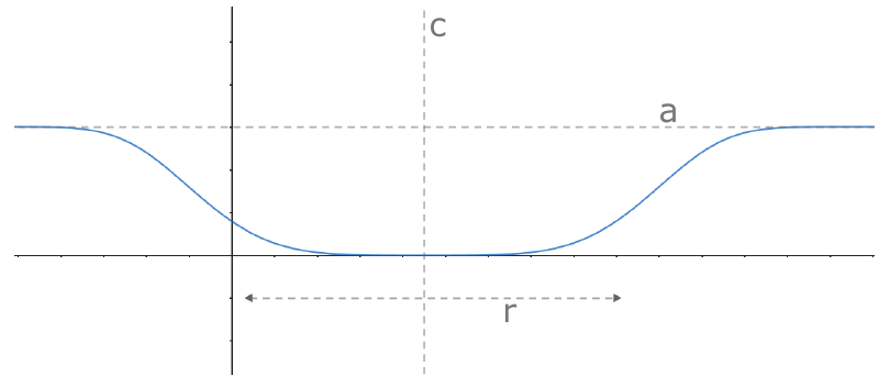
These three parameters allow to control the cost of a specific metric for every setup; for instance, the path slope can be very reasonable from -0.1 to 0.1, but outside that range the cost should become much higher since the path becomes very steep. However, for a T5 (a high difficulty trail), the range of acceptable values for the path slope can be broader, thus we should put a larger value of r for the path slope in the cost function when generating T5 trails.
We used machine learning to automatically determine the optimal values for these parameters. Since the pathfinding (e.g. Dijkstra’s algorithm) step is not differentiable, we cannot use techniques relying on gradient descent, such as neural networks. We used a genetic algorithm for this step.
Despite optimizations (such as generating paths on downsampled versions of the terrain), the graph generation and pathfinding steps can be slow for large terrains, causing the whole training pipeline to be very slow. We could only affort to train the GA for 15 generations with 200 individuals.
A final detail is the loss function that we use, e.g. how do we determine how good or bad a result is. For this, we decided to compare the results to a real reference: we generate a path between the start and end points of an existing path, then compare how different the two are. To compare two paths, we have two very different approaches:
- Fréchet distance: is used to measure the distance between curves in space (3D in our case). It computes the distance between two points at the point when it is maximal.
- Cost ratio: the Fréchet distance is not very well-suited to our problem, since (1) it only considers the maximum difference, ignoring any other similarity; (2) it will penalize paths that are spatially far away, without taking into account the terrain properties. The cost ratio addresses those issues by comparing the cost of the paths in the graph instead, ignoring spatial distance.
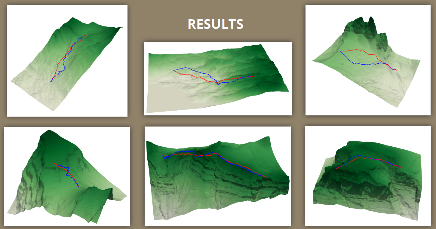
The image below shows some results of the path generation. In blue, the original trails from OpenStreetMap, in red, the generated ones (enforcing that the start and end points be the same). Generated trails, although adapting somewhat to the terrain, tend to go very straight from the start to the end points, in some cases creating not very plausible results, and showing there is still room for improvement in this step.
3. Network generation
Create a trail network connecting multiple Points of Interest.
The final step of the project is to scale the path generator to create a whole network of trails.
We are given a terrain surface and a set of Points of Interest that we want to be reachable by the trails.
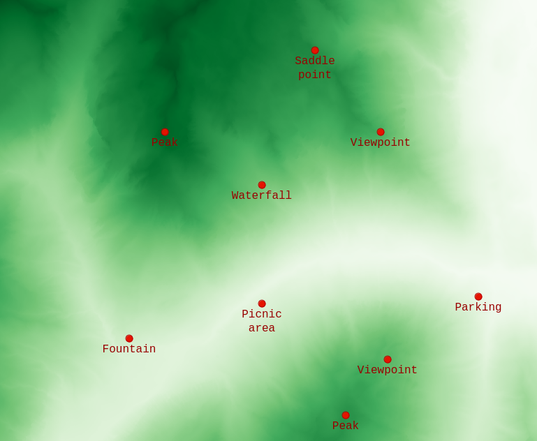
We approach this problem by generating all possible trails between paths, of all levels of difficulty (T1 to T5); we then prune the least suitable trails, ensuring that the remaining graph is still connected, until a user-defined threshold of path density.
However, generating all possible trails is computationally infeasible for large terrains with many PoIs. We thus simplify the task by previously computing a connectivity graph, based solely on 2D spatial distances between PoIs, and then only generate paths for those pairs of connected PoIs in the connectivity graph. There are many possible options to define the connectivity of PoIs, but we found the Delaunay triangulation to be the best option in terms of desireable properties for the final result.
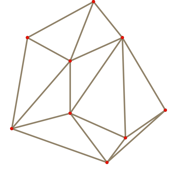
5 trails (T1 to T5) are then generated between each pair of connected PoIs. Then paths are pruned one by one according to their cost (a higher cost indicates a worse fit to the terrain, so it should be pruned first), except those that would create a disconnected graph (even if a path is not very good, it is still the best of all available options to connect the graph).
Some final post-processing steps are done to merge all the generated paths into a single network with intersections.

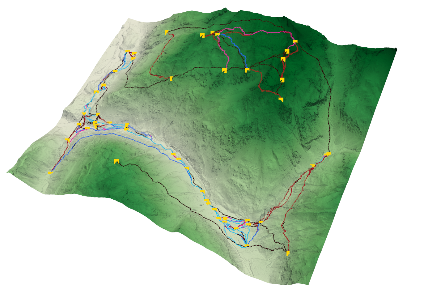
The final network presents some desireable properties. We see that places that are hard to reach are usually connected by a single path, and it is of high difficulty (black color). Trails that traverse easier terrains are usually of an easier difficulty (light and dark blue). There is also a higher density of paths in easier terrains, where more possibilities for paths exist.
Finally, through our pruning approach, we can also obtain more than one path connecting PoIs , which is also something we observe in reality, with high-difficulty trails usually taking steeper but more direct routes to reach the destination.
What’s next?
Development of the SENDA project goes on, and these results will be used for the next stages of the broader project. Regarding this particular work itself, there is the intention of continuing it, improving on its performance and polishing some details. The main areas to focus now are:
- Improve the results of the path generation: either increase the complexity of the edge cost function to allow for more expresiveness, or train longer (much longer); probably both. Optimizing the system to allow for faster training is very needed for the latter.
- Polish the system with a user friendly UI to control all the generation parameters.
- Explore how well these methods generalize to other contexts, for example, the difficulty classification and generation of ski pistes in mountainous terrain.